There’s a fine line between a well-formatted Microsoft Excel worksheet and one that’s full of issues that take time to fix. Whether you’re an Excel newbie or a seasoned pro, avoiding these formatting habits will ultimately speed up your workflow and ensure your spreadsheet works as expected.

6

Merging Cells

Picture this: you have a row in Excel where the same data applies to each cell. Rather than repeating the same value multiple times, you decide to click “Merge And Center” in the Home tab on the ribbon.

That looks great, right? However, formatting your data in this way is a sfouurefire way to give yourself and your coworkers a headache down the line.

Microsoft Excel works best when you have a consistent grid of individual cells placed in rows and columns, so merging cells disrupts this spreadsheet structure.

For example, if you add filter buttons to the top row of your data containing merged cells, and try to sort that data using these buttons, you’ll see an error message. The same happens if you click “Sort” in the Data tab on the ribbon.

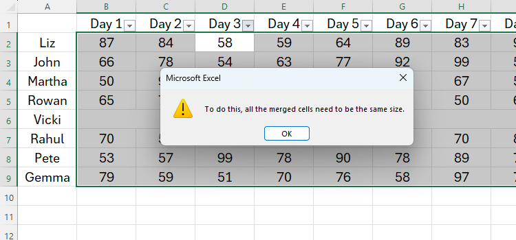
You’ll also face a similar issue if you try to paste data from an unmerged row to a merged row.

Luckily, there’s an alternative way to achieve a similar formatting outcome without sending Excel into a frenzy: the Center Across Selection tool.

Related

Don’t Merge and Center in Excel: Center Across Selection Instead

I was a loyal merger and centerer until I found this tool.

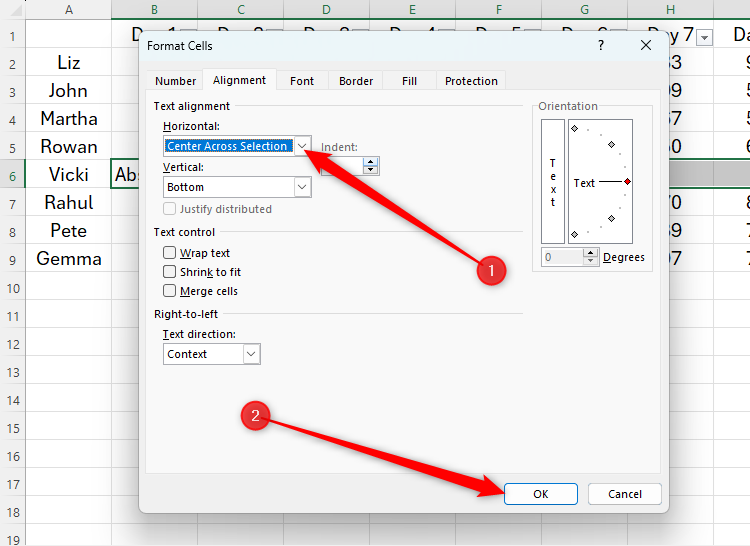
First, select the cells you would have previously merged, and click the dialog box launcher icon in the bottom-right corner of the Alignment Group in the Home tab. Alternatively, press Ctrl+1, and hit the Right Arrow key.

Next, expand the “Horizontal” drop-down menu, and click “Center Across Selection.” Then, click “OK.”

Now, although the cells look like they’re merged, their structure and integrity have been preserved. As a result, you can use the filters and copy and paste data between rows without triggering any error messages.

5

Center and Left-Aligning Numbers

When you enter text into a cell in Microsoft Excel, it aligns to the left, and when you enter a numerical value, it aligns to the right.

Related

Excel’s 12 Number Format Options and How They Affect Your Data

Adjust your cells’ number formats to match their data type.

As a result, you might choose to left-align the cells containing numbers to make your spreadsheet look tidier. On the other hand, you might select all the cells and apply center alignment to everything in your spreadsheet.

But stop there! There are good reasons why Excel automatically places numerical values to the right of a cell.

On the one hand, having all numbers aligned to the right makes them easier to read and compare than when they’re center-aligned.

On the other hand, numbers being right-aligned makes it easier to differentiate between different types of data. For example, if your spreadsheet is automatically left-aligning what you think is a number, there’s a good chance that it’s formatted as text, meaning formulas referencing that cell won’t work as expected.

So, avoid the temptation to change the alignment of numerical values in your spreadsheet!

4

Not Using a Recognized Date Format

When you enter a value into a cell that Excel recognizes as a date, the number format in the Number group of the Home tab will change to either Date or Custom.

However, if it tells you that the cell still has General number formatting, it means that what you’ve entered is recognized as text. As a result, you won’t be able to use the value in formulas, like working out the difference between two dates.

Related

What Are Date and Time Serial Numbers in Microsoft Excel, and Why Do They Exist?

Date and time calculations would be impossible without them.

To fix this, first, clear the cell by selecting it and pressing Delete. Then, press Ctrl+1 to launch the Format Cells dialog box, and click “Date” in the Category list of the Number tab. There, you’ll see the various date formatting options you can select to force Excel to see your value as a date.

Alternatively, click “Custom” in the Category list, and either choose one of the options in the list or type a different combination of Y, M, and D to represent years, months, and days, respectively:

After clicking “OK,” type the date using the structure you selected or created, and Excel will recognize the number format correctly.

3

Color-Filling Whole Columns or Rows

In this screenshot, the whole of column D is manually formatted with a blue cell fill to indicate that it contains the totals.

However, this means that you have more cells formatted than necessary, making your spreadsheet look untidy and slowing its processing speed.

Related

7 Ways to Speed Up Your Excel Spreadsheets

Don’t twiddle your thumbs waiting for Excel to respond.

Also, if you select some cells in the colored column and shift them to the right to insert more data, the formatting will become skewed.

The best alternative is to format your data as an Excel table, and adjust the table’s design to bold the right-most column.

To do this, select the data, and in the Home tab on the ribbon, click “Format As Table.”

Then, select a cell in the table, open the “Table Design” tab, and check “Last Column” in the Table Style Options group to bold the total column. You could also select the data and increase the font size for added emphasis.

However, if your data contains a dynamic array, this method won’t work because Excel tables can’t accommodate spilled arrays. Also, you might want to emphasize a different column.

Related

Everything You Need to Know About Spill in Excel

It’s not worth crying over spilled references.

In these scenarios, use conditional formatting. In this example, you want the cell in column E to turn blue when there’s a number in column A of the corresponding row.

So, select the whole of column E by clicking the column header, and in the Home tab on the ribbon, click Conditional Formatting > New Rule.

Then, click “Use A Formula To Determine Which Cells To Format,” and in the empty formula field, type:

=ISNUMBER($A1)

Next, click “Format” to select the fill color, and click “OK” to close the dialog boxes.

Because you told Excel to color the selected cells when the value in column A is a number, only the relevant cells are colored, and when you add more data to column A, the corresponding cell in column E adopts that formatting.

2

Using Different Fonts

When teaching people how to use Excel, I always emphasize the importance of consistency, and this is particularly true when it comes to font selection.

Mixing typefaces in Excel makes the spreadsheet appear cluttered, disorganized, and unprofessional, and can present challenges for people with reading difficulties.

Instead, choose a single sans-serif font that is easy to read, clearly differentiates between letters and numbers that might look the same in other fonts, and isn’t too stylistic. Aptos, Arial, Tahoma, and Verdana are good choices for readable and professional spreadsheets.

Related

Which Fonts Should You Use in Excel?

Optimize your data’s readability.

1

Formatting Tables Manually

In Microsoft Excel, you can apply manual formatting to data to increase its readability and make certain values stand out.

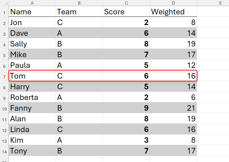
In this example, a border has been added between rows 1 and 2, the values in column C are bold, and every other row has been filled gray.

However, if you wanted to add data to row 13 or column D, you would need to duplicate the formatting manually.

What’s more, if you were to insert a new row in the middle of the data, the banded row formatting would be out of line.

In fact, formatting your table manually could cause many other issues down the line, all of which would take time to fix.

Instead, select your unformatted data, and in the Home tab on the ribbon, click “Format As Table.”

Related

Everything You Need to Know About Excel Tables (And Why You Should Always Use Them)

This could totally change how you work in Excel.

Then, in the Create Table dialog box, make sure the correct cells are selected, check “My Table Has Headers” if this is the case, and click “OK.”

Now, your data is reformatted as an Excel table, and in the Table Design tab, you can add and remove row banding, filter buttons, a total row, and various other options.

What’s more, when you add more rows and columns by clicking and dragging the table fill handle in the bottom-right corner, any table formatting will be automatically applied to these new cells.

Ultimately, when using Microsoft Excel, aim to make your spreadsheet easy to read and your data easy to manipulate. Avoiding the formatting habits discussed in this article will go a long way in helping you achieve this.