Copying data from an image into a Google Sheets file manually can be time-consuming and increases the chances of typos. Luckily, you can extract the information into your spreadsheet in just a few simple steps using the Optical Character Recognition (OCR) tool in Google Drive. Here’s how.

Points to Note Before You Start

Before you begin converting the text in your image to data in Google Sheets, here are some pointers that will help ensure the process works as expected:

• Make sure your image is clear: The better the quality of the picture, the better the conversion will be. If your image is a screenshot, this shouldn’t be too much of a problem. However, if you capture the picture with your phone or a camera, make sure it’s well-lit and not obscured by shadows. Also, try your best to have a steady hand to avoid blurriness.
• Use images with high-resolution text: The data in the picture must be at least 10px high.
• Ensure the image is the correct format: This process works with JPEG, PNG, TIFF, and GIF files. If your image is not one of these image file formats, be sure to convert it first.
• Don’t use overly large images: Google recommends that the file size be 2MB or smaller.
• Standard fonts work best: If the text or numerical data in the image is in an unusual font, the conversion might not work as well as you had hoped.
• Formatting may not be preserved: Be prepared to make manual changes to the data formatting once the conversion is complete.
• You need a Google account: In order to take advantage of this OCR conversion tool, you need to be signed in to your Google account.

Step 1: Upload the Image to Google Drive

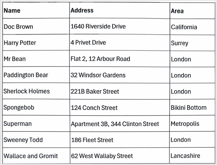
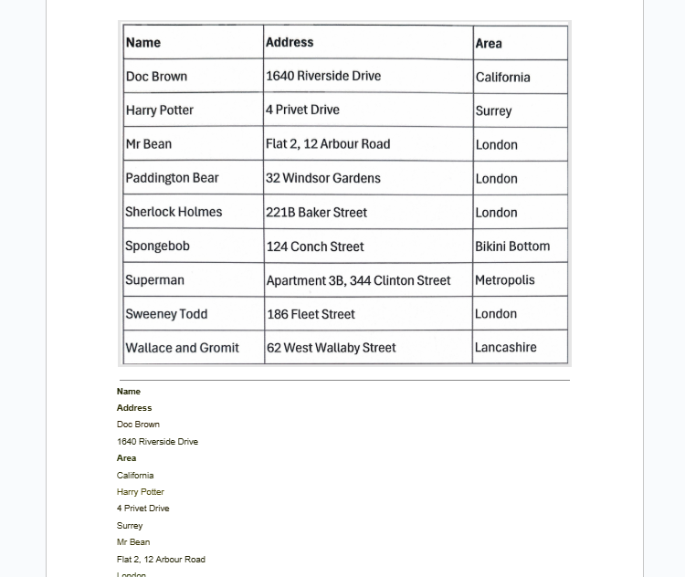
Let’s say you’ve downloaded this image—a screenshot of a PDF containing various names and addresses in PNG format—and you want to extract and edit the data in Google Sheets.

Because the file is a PNG image, you can’t simply select and copy the text, as the file doesn’t contain any “real text” data—only image data. You might also encounter the same scenario if you copy data from a website—if it was uploaded as an image, there won’t be any real text to simply copy and paste into Google Sheets.

Instead, upload the image to Google Drive. Before you do this, make sure the image is the right way up.

Related

How to Rotate Images on Windows 11

Rotate photos using the built-in apps like File Explorer, Photos, and Paint.

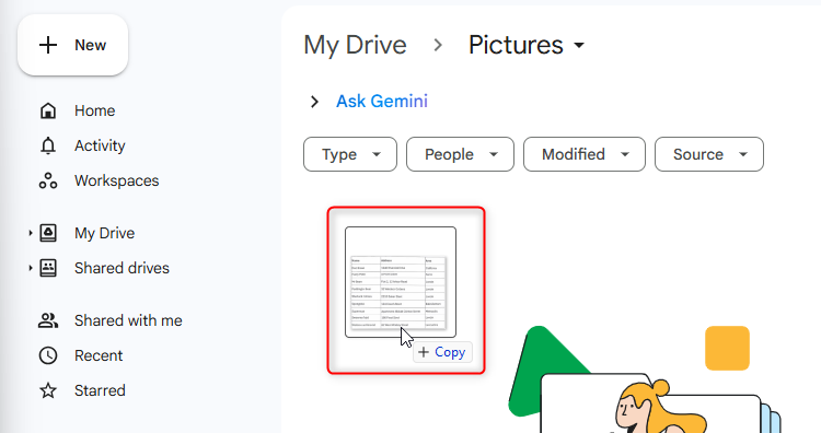
Then, sign in to Google Drive, and click and drag the file to the relevant Google Drive folder.

Alternatively, click “New” in the top-left corner, select “File Upload,” and locate and upload the image you want to convert.

Step 2: Open the Image in Google Docs

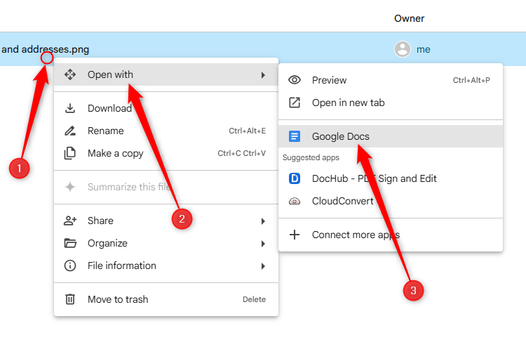
Now that your image has been uploaded to Google Drive, it’s time to kick the conversion process into action. To do this, right-click the file, hover over “Open With,” and select “Google Docs.” Yes, you ultimately want the data to be in Google Sheets, but this is a necessary step to take first.

At this point, Google Docs opens in a new tab, with the original image at the top of the document and the extracted data underneath.

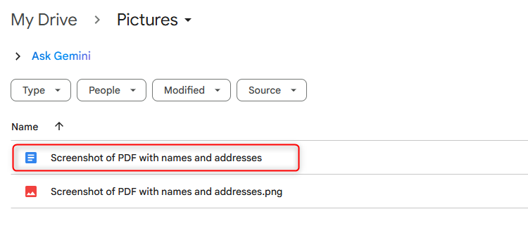
Also, if you head back to the Google Drive folder containing the image, you’ll see that the Google Docs file you just created is saved in the same location with the same name.

Related

I Paid for Google’s Drive Storage. Here’s Why I Don’t Regret It

The convenience is worth 2 dollars a month.

Step 3: Review the Data and Make Necessary Changes

While OCR is generally accurate, depending on how the data in the original image is laid out, it isn’t always perfect. So, take some time to review the data in the Google Docs file you just created.

In this example, the column headers in the image are inserted in random positions in the list of extracted data, so I’ll remove these for now and add them again later on when I edit the data in Google Sheets.

Also, towards the end of the list, the addresses of Spongebob, Superman, and Sweeney Todd have been mixed up, so I need to reorganize this information so that the data is easier to work with in the next step.

Step 4: Copy and Paste the Data Into Google Sheets

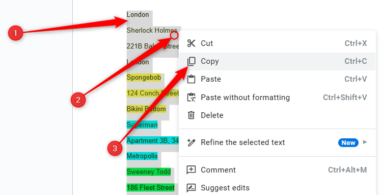
Now that the data is correctly ordered and organized, it’s ready to be moved over to Google Sheets. To do this, select the data, right-click anywhere in the selected area, and click “Copy.”

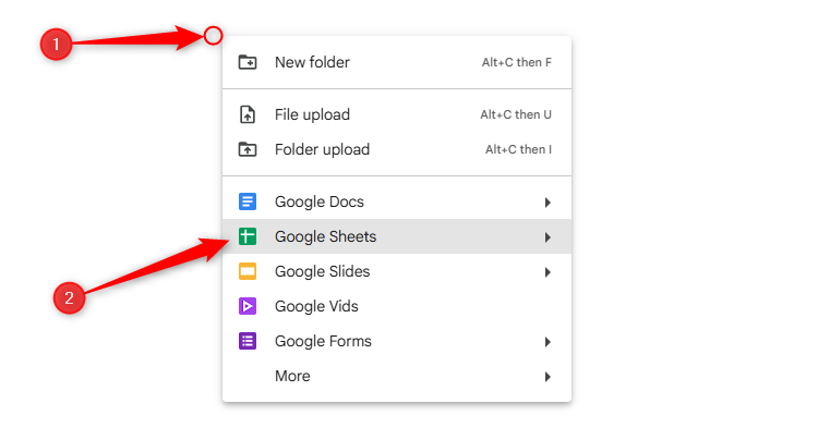
If you want to insert the data into a new spreadsheet, right-click the white space in the relevant Google Drive folder, and click “Google Sheets.”

On the other hand, if you already have the Google Sheets file set up, locate and open it.

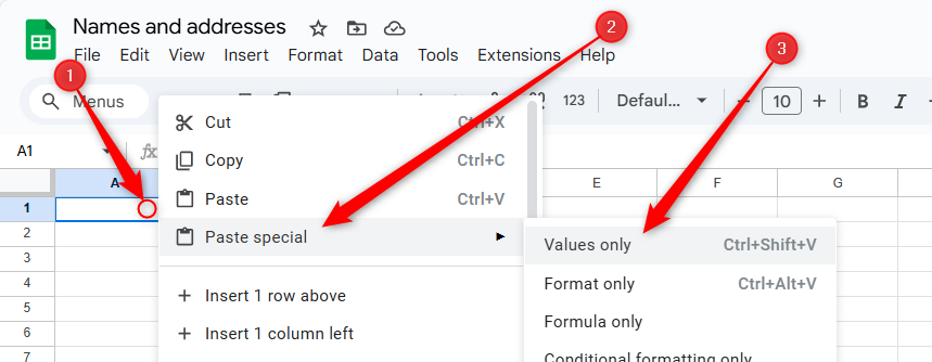
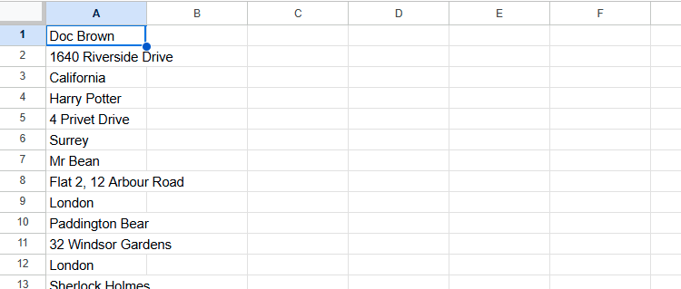
Next, right-click the cell where you want the first part of the copied data to be pasted, hover over “Paste Special,” and click “Values Only.” Pasting the data as values only removes all the formatting, including any line-spacing properties automatically adopted by Google Docs, so that you can work with a clean set of data.

Step 5: Format the Data

The final step in the image-to-data conversion is to format the data in Google Sheets, so that it appears and behaves exactly how you want it to.

In my case, the list is set in one column, but I want names, addresses, and areas to be in three separate columns.

There are various ways to transform the dataset accordingly, but in my case, I’m going to use the TRANSPOSE function, which turns horizontal data into vertical data (and vice versa).

Related

Convert a Row to a Column (or Backwards) in Google Sheets

Don’t switch your data manually!

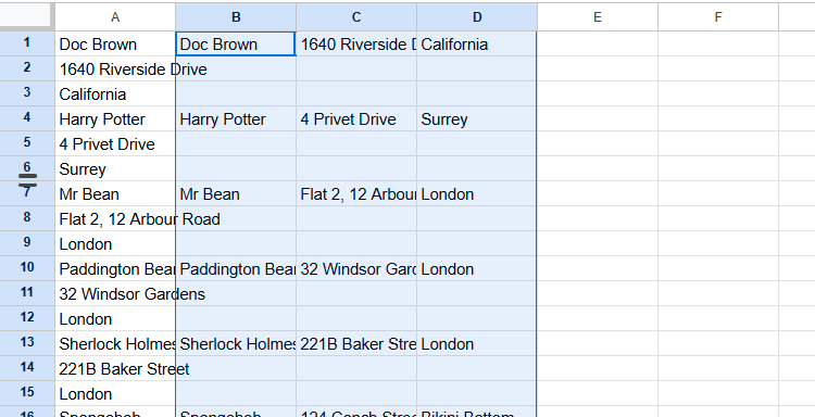
If you want to do the same, in cell B2, type:

=transpose(A1:A3)

and press Enter.

Now, because a new name appears in every third row, select cells B1 to B3, and double-click the fill handle to duplicate the TRANSPOSE formula in the relevant cells in column B.

Next, select all the newly transposed cells, press Ctrl+C to copy them, and press Ctrl+Shift+V to paste the values only. This detaches the data from the original one-dimensional list, meaning you can delete it, safe in the knowledge that you won’t lose any of your transposed data.

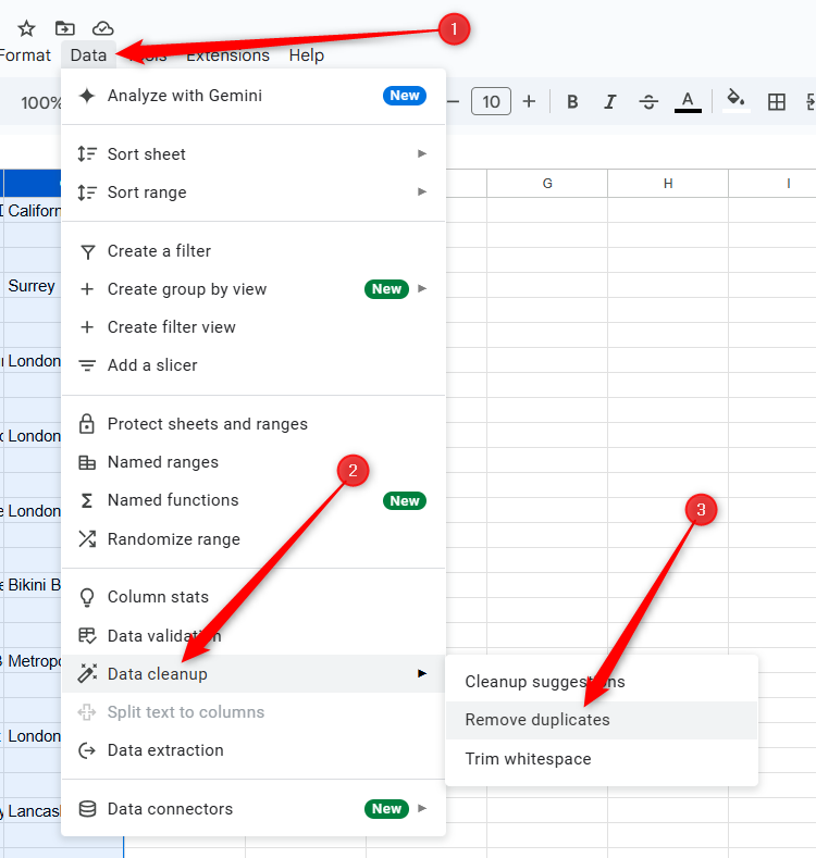
Now, after right-clicking the column A header and selecting “Delete Column,” you need to remove the blank rows. To do this, select all the columns containing the data, and in the Data tab, hover over “Data Cleanup,” and click “Remove Duplicates.”

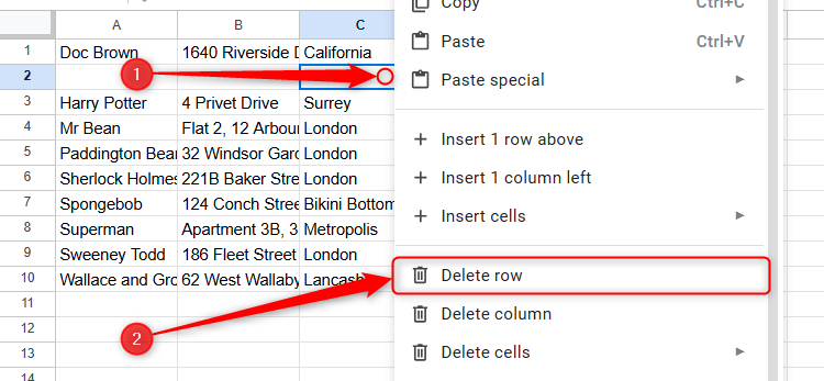
This will leave one blank row, which you can delete manually by right-clicking any cell in that row, and clicking “Delete Row.”

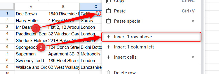
Finally, to reinsert the column headers, right-click any cell in row 1, click “Insert 1 Row Above,” and type the headers as necessary.

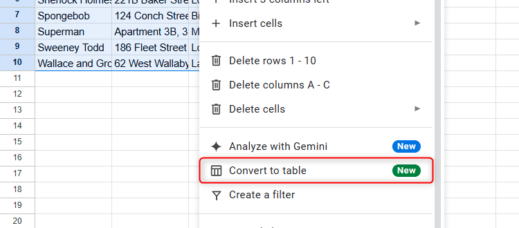
You can now convert the data to a formatted Google Sheets table by selecting all the cells (including the column headers), right-clicking the selection, and clicking “Convert To Table.”

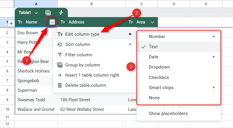
Then, click the down arrows in each column header and hover over “Edit Column Type” to ensure the correct data type is assigned to each field, and your converted data is ready for use in your Google Sheets spreadsheet!

Related

Google Sheets vs. Microsoft Excel: Which Should You Use?

Yes, they’re both spreadsheet platforms, but they’re actually very different.