Microsoft Excel’s CHOOSECOLS and CHOOSEROWS functions are a game-changer if you want to quickly extract specific columns or rows from your data without nesting several functions in your formula. What’s more, they’re dynamic functions, meaning they adapt to changes in your dataset.

The CHOOSECOLS and CHOOSEROWS Syntaxes

Excel’s CHOOSECOLS and CHOOSEROWS functions are like twins: their DNAs are very similar, but they’re separated by subtle differences. The same can be said for their syntaxes.

Here’s the syntax for CHOOSECOLS:

=CHOOSECOLS(a,b,c,…)

And here’s the syntax for CHOOSEROWS:

=CHOOSEROWS(a,b,c,…)

In both cases,

• a (required) is the original array that contains the columns (CHOOSECOLS) or rows (CHOOSEROWS) you want to extract,
• b (required) is the index number of the first column (CHOOSECOLS) or row (CHOOSEROWS) to be extracted,
• c (optional) represents the index numbers of any additional columns (CHOOSECOLS) or rows (CHOOSEROWS) to be extracted, each of which must be separated by commas.

You might be thinking that these functions sound very similar to the TAKE function. However, where TAKE lets you extract the first or last x columns or rows, or a single column or row from elsewhere in a named table, CHOOSECOLS and CHOOSEROWS let you extract any number of columns in any order from anywhere in your data.

Related

How to Use TAKE in Excel to Extract Data

Extract specific data from your Excel table.

Example 1: Extracting the First and Last Column or Row From a Table

I’ve already lost count of the number of times I’ve used CHOOSECOLS and CHOOSEROWS to extract the first and last column or row from a table. This is particularly handy if the first column or row is a header, and the last column or row contains totals.

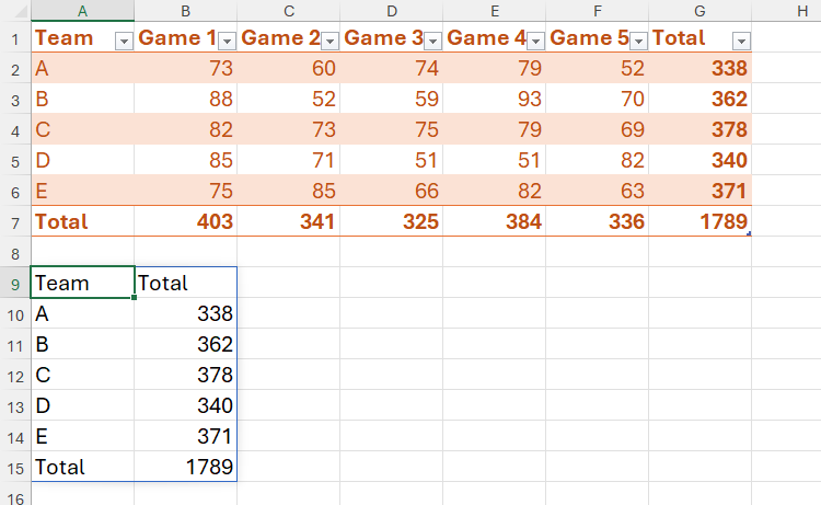
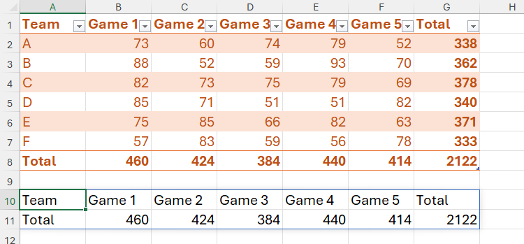
Imagine you’re an administrator for a local sports league, and you’re producing a report that summarizes the points scored by five teams across five games.

The first dataset you want to generate will tell you the total number of points scored overall by each team. To do this, in a blank cell, type:

=CHOOSECOLS(T_Games[#All],1,-1)

where

• CHOOSECOLS is the function you want to use, since you’re extracting the data from the Team and Total columns,
• T_Games is the name of the table where the array is stored, and [#All] tells Excel that you want to include the header and total rows in the result,
• 1 is the first column (in this case, the column named “Team”), and
• -1 is the last column (in this case, the column named “Total”)

and press Enter.

Here’s the result you get when you press Enter, and this data can be duplicated on another sheet in the same workbook, such as a dashboard tab, or copied and pasted as text in an email or Word document.

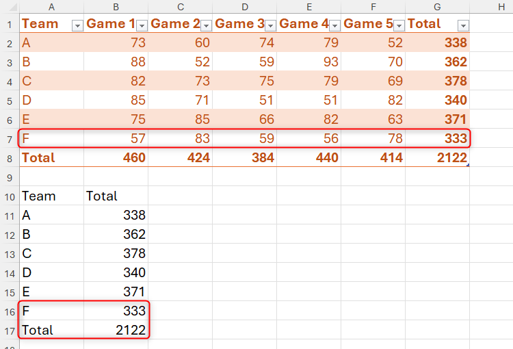
Now, even if more data is added, the result—including the Total row—updates accordingly.

The next report you want to generate will show the number of points scored in each game (rows 1 and 8).

So, in a blank cell, type:

=CHOOSEROWS(T_Games[#All],1,-1)

and press Enter. Remember that adding [#ALL] after the table name in the formula forces Excel to count the header and total rows when addressing the index numbers.

Example 2: Extracting Columns From More Than One Range

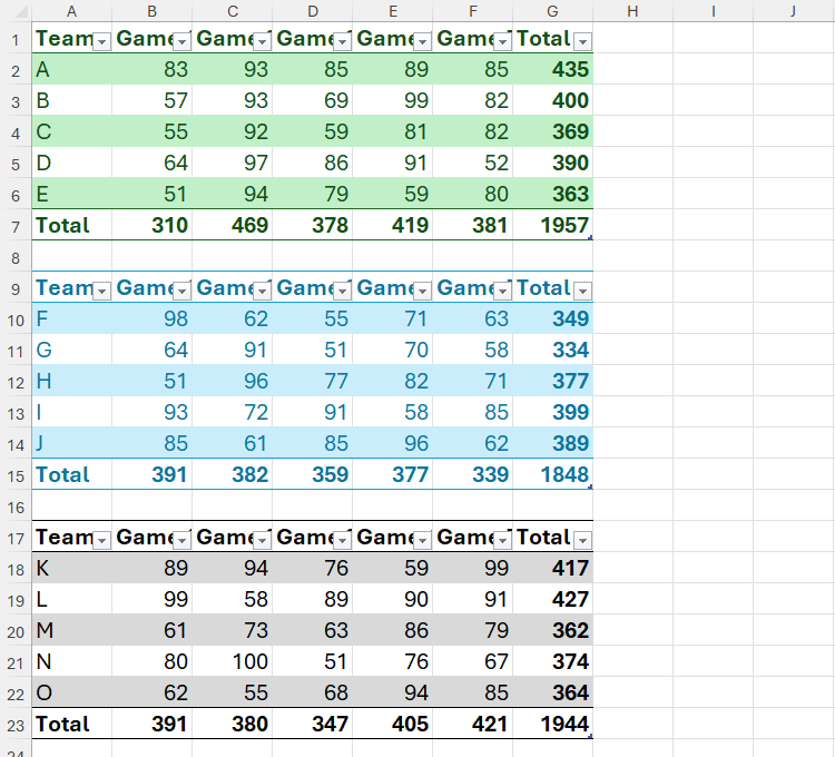
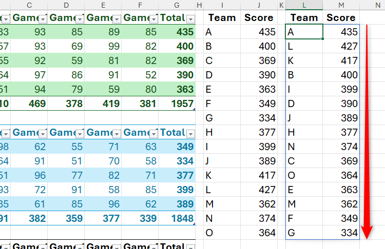
Now, let’s say you have this spreadsheet, and your aim is to produce a list containing the total scores of each team across Leagues 1 (green), 2 (blue), and 3 (gray).

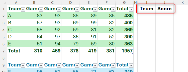
This time, you don’t want Excel to extract the column headers and row totals, since you’re going to nest the VSTACK function within the CHOOSECOLS formula to stack the three tables directly on top of each other. So, in cells I1 and J1, create the column headers manually.

Related

How to Combine, Reshape, and Resize Arrays in Excel

Take control of the arrays in your spreadsheet and arrange them as you please.

Then, in cell I2, type:

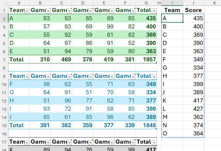
=CHOOSECOLS(VSTACK(League_1,League_2,League_3),1,-1)

where

• CHOOSECOLS is the function you’ll use to extract columns,
• VSTACK lets you combine the results vertically,
• League_1,League_2,League3 are the names of the tables that represent the arrays, and the absence of [#ALL] after the table names tells Excel not to include the header and total rows in the result,
• 1 tells Excel to extract the first column (“Team”) from each array, and
• -1 tells Excel to extract the last column from each array (“Total”)

and press Enter.

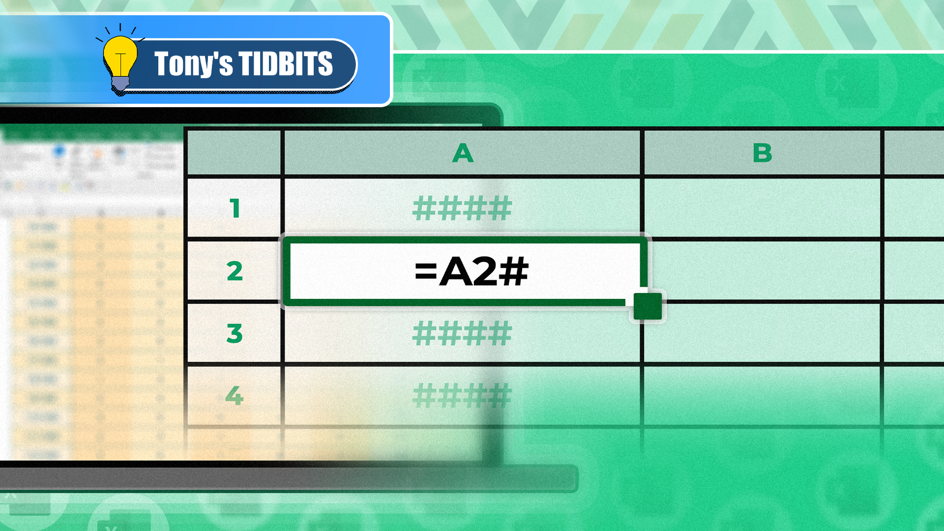
At this point, you could go one step further and sort the result in descending order by typing:

=SORTBY(I2#,J2:J16,-1)

into cell L2, and pressing Enter.

Related

You Need to Know What the Hash Sign Does in Excel Formulas

Smash the hash in a flash!

Example 3: Using CHOOSECOLS With Data Validation and Conditional Formatting

So far, I’ve shown you the benefits of using CHOOSECOLS and CHOOSEROWS to extract the first and last columns and rows from an array. However, this time, I’ll show you how you can use CHOOSECOLS to extract other columns, and combine this with additional Excel tools to make your spreadsheet stand out.

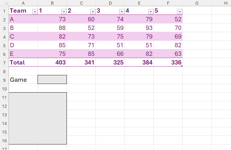
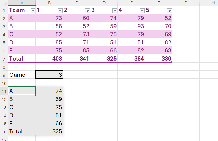
This spreadsheet shows five teams’ scores over five games, including the total points scored in each game in the total row. Your aim here is to produce a result that shows each team’s score and the overall total in cells A11 to B15 for a game number you will enter into cell B9.

First, type a game number into cell B9, so that you have something to work with when you generate your CHOOSECOLS formula. Then, in cell A11, type:

=CHOOSECOLS(T_Scores[[#Data],[#Totals]],1,B9+1)

where

• CHOOSECOLS is the formula used to extract columns,
• T_Scores is the name of the table, and [[#Data],[#Totals]] tells Excel to include the data and the totals in the result, but not the header row,
• 1 represents the first column (“Totals”), and
• B9+1 tells Excel that the second index argument is represented by the value in cell B9, plus one. The reason you need to include +1 here is because the game numbers start in the second column of the table. As a result, typing 3 into cell B9 extracts the data from the fourth column of the table, which is game 3.

Although typing the game number into cell B9 works well, if you or someone else accidentally enter an invalid number, the CHOOSECOLS function will return a #VALUE error.

This is a good case for using data validation in cell B9 to create a drop-down list of the available game numbers.

Related

How to Add a Drop-Down List to a Cell in Excel

It beats typing in the same options 200 different times manually.

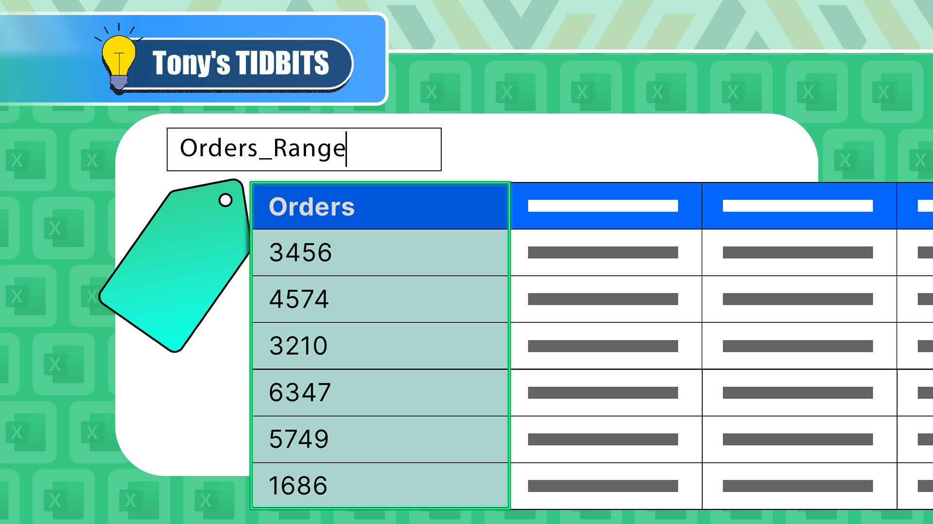
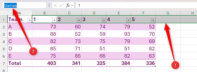
My preferred way to do this for a header row in an Excel table is to first select all the relevant cells, plus a few extra to allow for growth, and name the range in the name box in the top-left corner of the Excel window. Notice how I’ve not selected the column header “Team,” because I don’t want this to appear in the game drop-down list in cell B9.

Related

I Always Name Ranges in Excel, and You Should Too

Tidy up your Excel workbook.

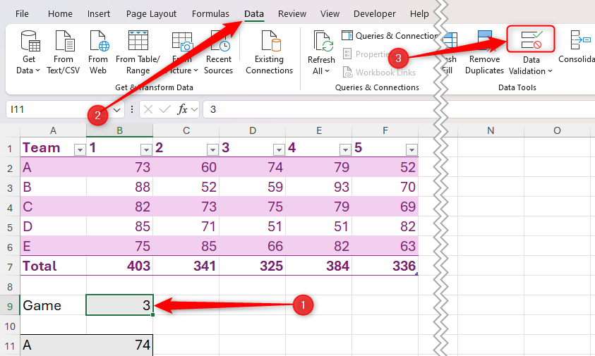
Next, select cell B9, and click the top half of the “Data Validation” button in the Data tab on the ribbon.

Now, in the Data Validation dialog box, select “List” in the Allow field, make sure “Ignore Blank” is checked, type an equal symbol (=) followed by the name you just gave to the column header range, and click “OK.”

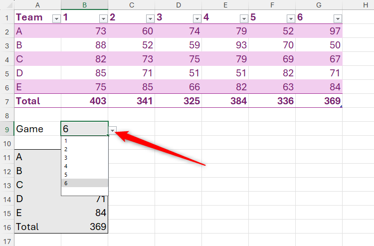
You can now click the drop-down arrow in cell B9 to select a valid game number, safe in the knowledge that even if you add extra columns to your table, CHOOSECOLS and the named range in data validation will work together to update the available options accordingly.

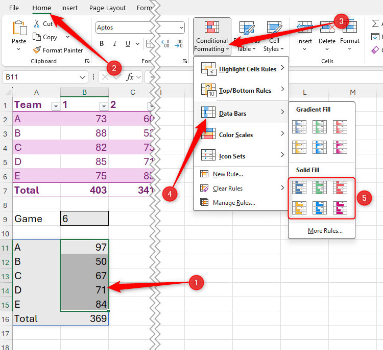
Finally, to visualize your data even further, select cells B11 to B15, and in the Home tab on the ribbon, click “Conditional Formatting,” hover over “Data Bars,” and choose a solid fill color.

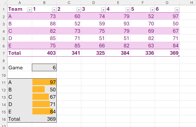
As a result, not only have you extracted specific columns from your data using CHOOSECOLS, but you’ve also made the result dynamic by adding a drop-down list, and you’ve formatted the data to add visual clarity.

CHOOSECOLS and CHOOSEROWS produce dynamic arrays, meaning the result spills out from the cell where you entered the formula. As a result, before you enter your formula, make sure there’s enough room in your spreadsheet—otherwise, you’ll get the dreaded #SPILL! error. Also, since dynamic arrays and formatted Excel tables don’t mix, if you want to format the result, you’ll have to do so manually or by using conditional formatting.