The CHOOSECOLS and CHOOSEROWS functions in Google Sheets are ideal for quickly extracting specific columns or rows from your data without creating confusing nested formulas. What’s more, since they’re dynamic functions, they adapt to changes in the source data.

The CHOOSECOLS and CHOOSEROWS Syntaxes

Once you work out how to use one of these two functions in Google Sheets, you’ll have a good understanding of how the other one works.

This is the syntax for CHOOSECOLS:

=CHOOSECOLS(a,b,c)

And here’s the syntax for CHOOSEROWS:

=CHOOSEROWS(a,b,c)

Here’s what each argument represents:

If any of the index numbers are zero or exceed the number of columns or rows in the array, Google Sheets will return the #VALUE! error.

Related

The Beginner’s Guide to Google Sheets

Find out how to do everything from sharing Sheets to automating tasks with macros.

Example 1: Extracting the First and Last Columns or Rows

Since I learned how the CHOOSECOLS and CHOOSEROWS functions work, I’ve used them endlessly to extract the first and last columns or rows from my data. This is a particularly handy trick if the first column or row is a header, and the last column or row contains totals.

Extracting the First and Last Columns

In this example, let’s imagine you’re a business administrator, and you want to create a report that summarizes the number of products sold by each shop in the first two quarters of the year.

To do this, in a blank cell, type:

=CHOOSECOLS(Sales[#ALL],1,-1)

where

• CHOOSECOLS is the function you need to use to extract data from the Shop and Tot columns,
• Sales is the name of the table containing the array, and [#ALL] tells Google Sheets that you want the header row to be included in the result,
• 1 indicates that you want to extract the first column (in this case, the Shop column), and
• -1 indicates that you want to extract the last column (in this case, the Tot column).

Here’s the result when you press Enter:

Notice how, even though you only typed the formula into cell J1, the result has spilled from that cell to cell K12 to accommodate the number of columns and rows in the result.

Also, because the source data is in a structured table, if the data changes, so does the result of the CHOOSECOLS function. This is also true if further columns or rows are added to the dataset.

Now, you can duplicate the summary data on another Google Sheets spreadsheet (such as a dashboard tab) or a Google Docs document.

Extracting the First and Last Rows

By the same token, pulling the first and last rows is handy for generating horizontal summaries of your data.

Using the same example as before, including the added Shop K, let’s say you now want to summarize the total number of products sold each month.

In a blank cell, type:

=chooserows(Sales[#ALL],1,-1)

and press Enter. As in the last example, adding [#ALL] after the table name tells Google Sheets that you want the header row to be counted as row 1 in the index lookup.

Example 2: Extracting Columns From More Than One Range

In Example 1, we extracted specific columns and rows from individual ranges. However, you can combine CHOOSECOLS with the VSTACK function to combine extractions from more than one range at the same time.

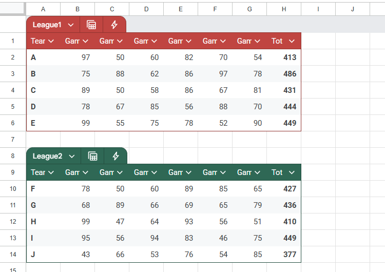
Here, you plan to generate a list of the total scores of each team in League 1 (red) and League 2 (green).

The first thing to note is that you don’t want to extract the column headers, since you want to stack the data from each table, one directly on top of the other. If you include the column headers, they’ll appear at the top of both datasets in the result, thus removing the sense that you’re looking at a combined dataset.

As a result, in cells J1 and K1, type the column headers manually.

Then, in cell J2, type:

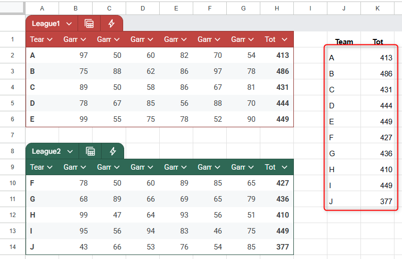
=CHOOSECOLS(VSTACK(League1,League2),1,-1)

where

• CHOOSECOLS tells Google Sheets that you want to extract certain columns,
• VSTACK combines the result vertically (hence the “v” in the function’s name),
• League1,League2 are the arrays that contain the columns, and [#ALL] not being included within the formula tells Google Sheets not to include header rows,
• 1 extracts the first column (Team) from each array, and
• -1 extracts the last column (Tot) from each array.

When you press Enter, here’s the result you get:

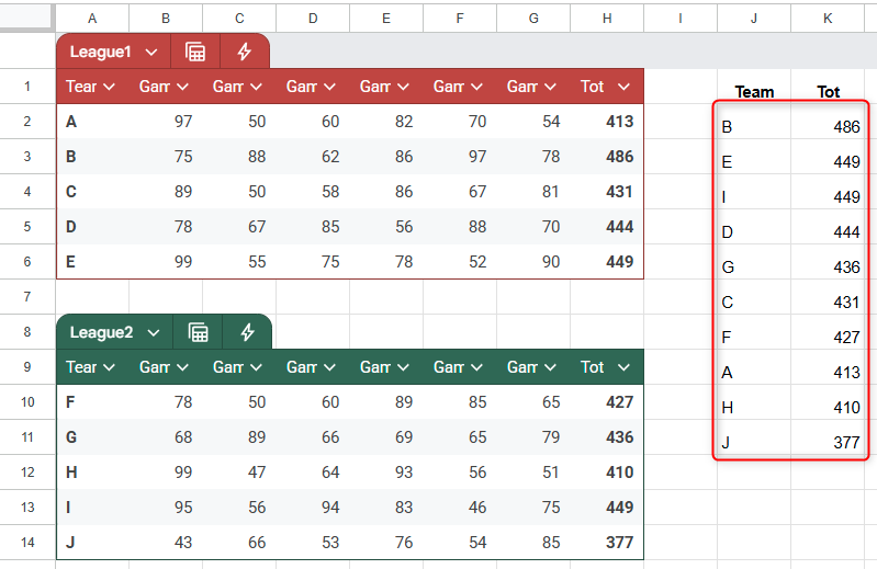
You could go one step further and nest the whole formula inside the SORT function, so the summary table displays the teams in order of their overall scores.

Related

9 Basic Google Sheets Functions You Should Know

Get familiar with the basic functions you need for your spreadsheet.

To do this, double-click the cell where you previously typed the CHOOSECOLS-VSTACK combination, and add the following SORT arguments:

=SORT(CHOOSECOLS(VSTACK(League1,League2),1,-1),2,FALSE)

where

• SORT is the function that sorts a range based on a specified column,
• 2 tells Google Sheets to sort the range by the second column, and
• FALSE indicates that the data should be sorted in descending order.

Impressively, if any values in the original dataset change, the summary table adjusts accordingly. Here, changing Team H’s Game 6 score from 51 to 89 promotes them from ninth position to fourth position.

Example 3: Making the CHOOSECOLS and CHOOSEROWS Functions Dynamic

So far, I’ve shown you how to use CHOOSECOLS and CHOOSEROWS to extract the first and last columns and rows from an array in Google Sheets. However, in this final example, I’ll show you how to extract other columns or rows dynamically by referencing cells—rather than using hard-coded index numbers—in the arguments.

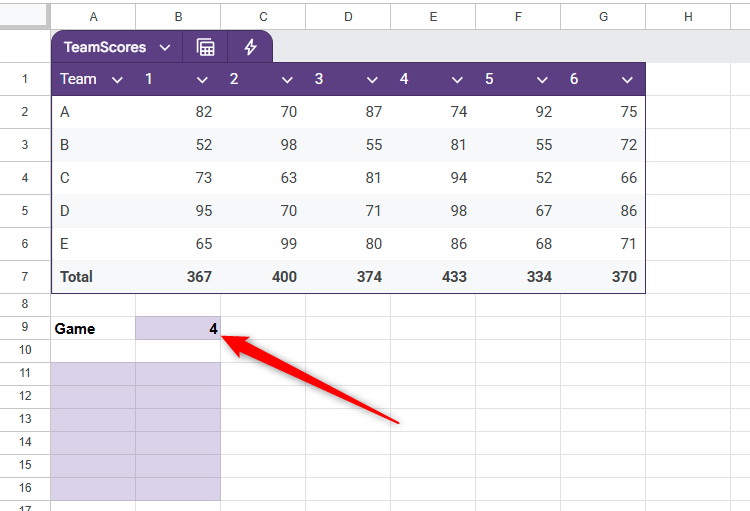
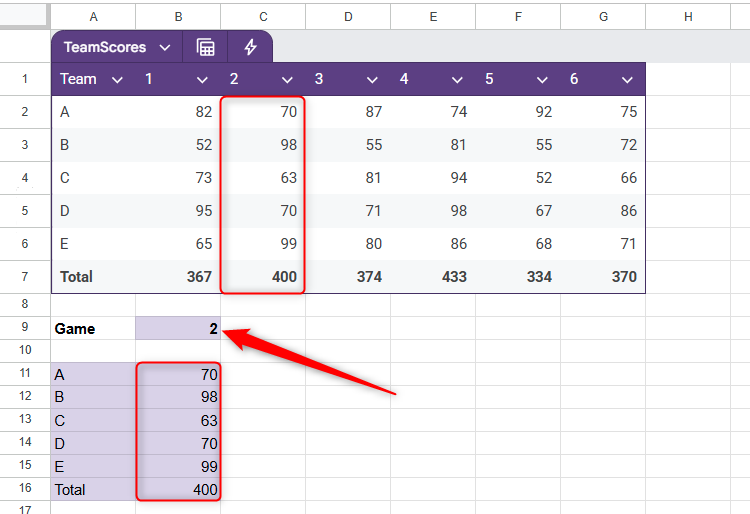
This Google Sheets table shows five teams’ scores over six games, as well as the combined total for each game, and your aim is to produce a summary according to the game number you specify in cell B9. First, type a game number into this cell so that you have something to work with when you generate your CHOOSECOLS formula.

Then, in cell A11, type:

=CHOOSECOLS(TeamScores,1,B9+1)

where

• CHOOSECOLS tells Google Sheets that you’re going to extract certain columns,
• TeamScores is the name of the table containing the data you want to extract,
• 1 is the index number for the Team column, and
• B9+1 tells Google Sheets that the second index argument is calculated by adding 1 to the value in cell B9. The reason you need to include +1 here is because the game numbers start in the second column of row 1, not the first. As a result, typing 4 into cell B9 extracts the data from the fifth column of the table, which is game 4.

Here’s what you get when you press Enter:

Now, type a different game number into cell B9 to see the result update accordingly.

Pro Tip: Add a Data Validation Rule

Although typing the game number into cell B9 works exactly as expected in making the CHOOSECOLS function dynamic, if an invalid number is entered, you’ll be abruptly met with a #VALUE! error. So, to prevent this from happening, you can use data validation to control the cell input parameters.

Related

How to Restrict Data in Google Sheets with Data Validation

Limit data inputs in a Google Sheets spreadsheet.

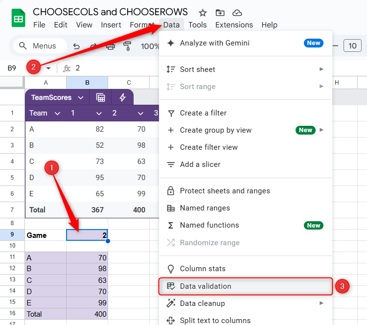
To do this, select cell B9, and in the Data tab, click “Data Validation.”

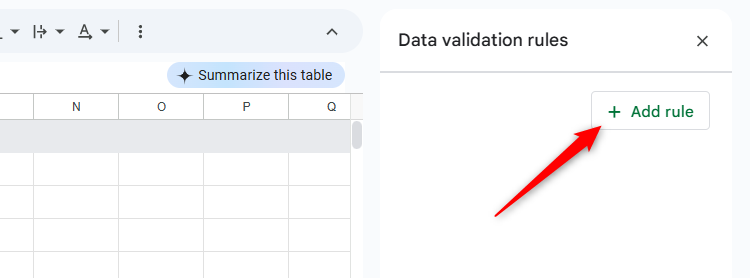
Then, in the Data Validation Rules pane on the right-hand side, click “Add Rule.”

Next, in the Criteria field, select “Dropdown,” and type the first possible input for this cell into the text field. Then, click “Add Another Item,” and repeat this process until all the inputs are stated. When all the options are listed, click “Done.”

Now, head back to cell B9, click the drop-down arrow, and select a different game number to see the result update accordingly.

The CHOOSECOLS and CHOOSEROWS functions in Google Sheets produce dynamic arrays, meaning the result spills out from the cell where you entered the formula. As a result, you must ensure there’s enough room in your spreadsheet before you enter your formula. Otherwise, you’ll see a #REF! error.