Excel sheets can get messy, especially if multiple people work on them or data is imported from other sources. This can lead to inconsistencies, duplicates, and formatting issues. Over time, I’ve picked up a few tricks that turn even the worst chaos into something clean, organized, and actually useful.

6

Clean Up the Formatting

An Excel sheet with inconsistent formatting can look ugly. You can use the Format Painter to copy formatting from one part of the sheet and paste it into another, making it uniform.

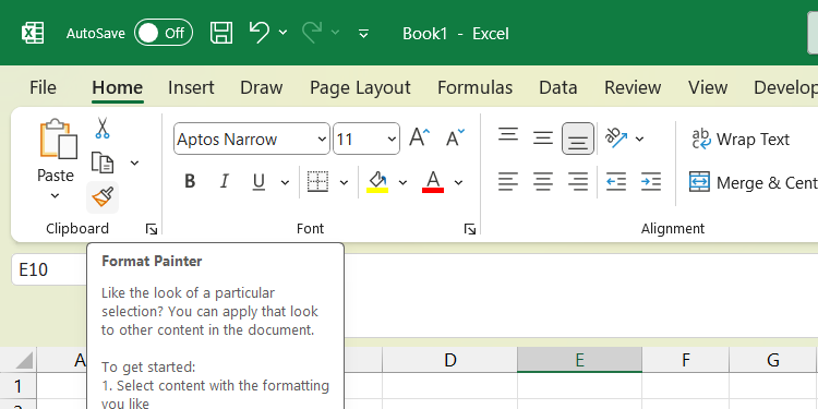
To use the Format Painter, select a formatted cell and click Format Painter (the paintbrush icon) in the Clipboard section of the Home tab to copy its formatting. The cursor will become a brush with a plus sign when the Format Painter is on. Afterward, click and drag to select the range of cells to which you want to apply the formatting.

After applying formatting, the Format Painter will be deselected, meaning you have to repeat the steps above to consistently format other parts of the sheet. To prevent this from happening, double-click Format Painter so it remains selected after applying the formatting. Click Format Painter again or press ESC to deselect it.

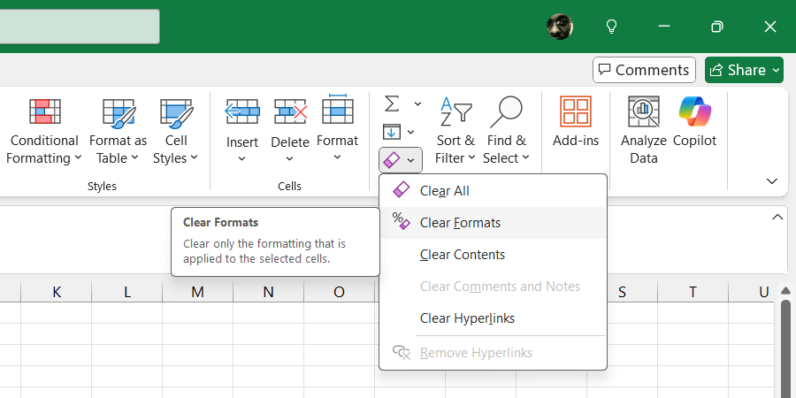
You might also just want to remove the formatting altogether if it doesn’t look good. To do that, select the cells with the formatting and click Clear > Clear Formats in the Editing section of the ribbon.

5

Trim Unnecessary Spaces

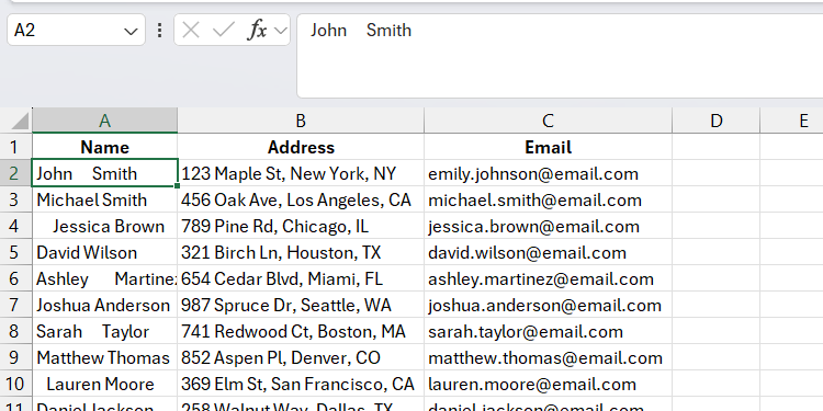
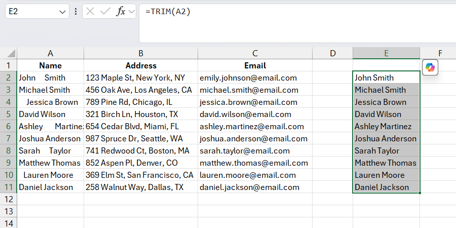
Another thing that doesn’t look good in an Excel sheet is leading, trailing, and multiple spaces. For example, instead of a name appearing as “John Smith,” it might be “John Smith” or ” John Smith,” which can make reporting and analysis inaccurate. You can fix these issues with the TRIM function in Excel and a helper cell.

For instance, if the range starts at cell A1, enter the following formula in a blank cell (the helper cell in this case) to get rid of any unnecessary spaces in the value in A1:

        =TRIM(A1)
    

Afterward, drag the handle of the helper cell to the adjacent cells to fill the other cells. Excel will intelligently detect that you want to trim spaces from the cells next to A1 and so on, and create more helper cells.

Now copy the values in the trimmed range and paste them into the original to replace the extra spaces.

Related

8 Little-Known Excel Functions That Can Save You Tons of Work

Your Excel game is about to go pro with these sneaky shortcuts.

4

Fill Empty Cells With Values

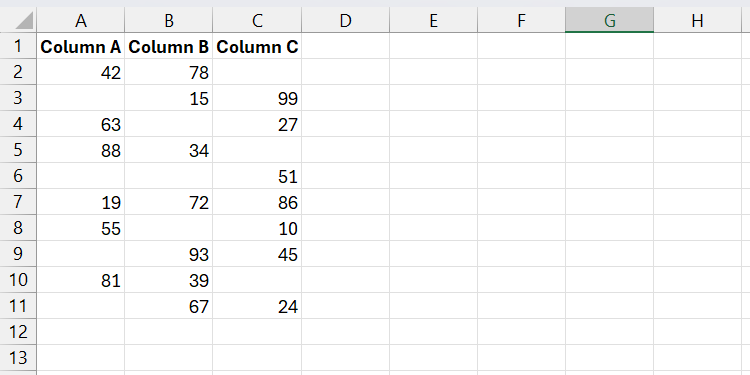
If the Excel sheet has empty cells, there are several ways you can find them and ensure they have a value. My favorite way is the Go to Special feature, which is an autofill trick in Excel. It will allow you to insert a value in all the blank cells at once or fill them in one by one for more precision.

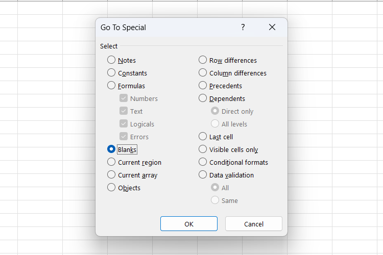
To use it, select the range with the blank cells and click Find & Select > Go to Special in the ribbon of the Home tab to open the Go To Special dialog box. Alternatively, you can press Ctrl + G.

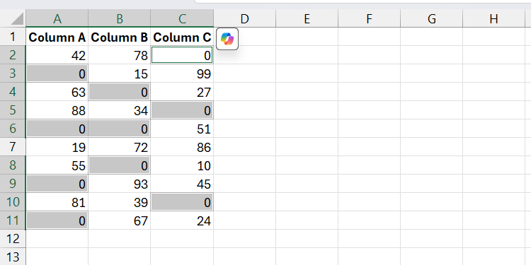
Tick the Blank radio button and then click OK to select all the blank cells in the range.

To fill all the blank cells at once, enter a value in the first highlighted cell and then press Ctrl + Enter. All the cells will then be filled with that value.

If the cells require different values, enter a value in the blank cell and press Tab to move to the next one until you have filled all of them.

3

Remove Duplicate Data

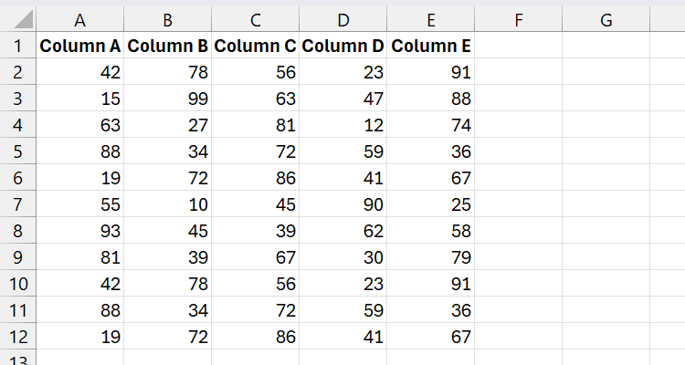
As you examine your Excel sheet, you might find that it contains duplicate rows. If there are many of them, chances are your human brain can miss a few. This can give you false insights when you analyze the data.

You can save your sanity by using conditional formatting to highlight them and take a closer look. But the easiest way to get rid of them is to use the Remove Duplicates tool.

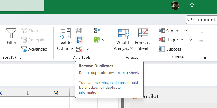
To use it, select the range with the duplicate rows, select the Data tab, and click Remove Duplicates in the Data Tools section of the ribbon.

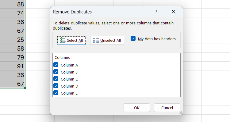
In the Remove Duplicates dialog box, you will see where all the duplicates are. Click OK to remove them.

2

Ensure Consistent Text Case

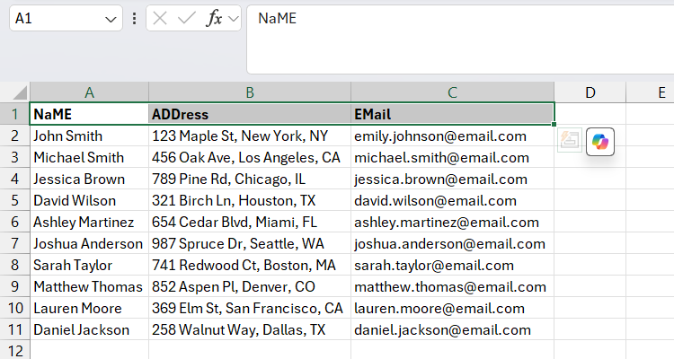
Consistent text case, whether uppercase, lowercase, or first letter capitals, is essential for a professional-looking sheet. Fixing inconsistent cases one by one can be time-consuming, depending on how big the sheet is. Luckily, you can easily fix it with functions like UPPER, LOWER, and PROPER in combination with a helper cell.

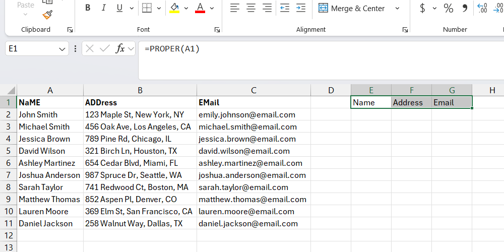
Take a look at the table below that we will be using for our example. To fix this, you need to convert the text in A1 (the starting header) into a helper cell and then apply it to the rest of the cells in the header.

To do this, select a blank cell and enter the following formula:

        =PROPER(A1)
    

Now, drag the fill handle to the adjacent cells in the row—you will see that Excel will intelligently fill it with data from A2, A3, and so on. Afterward, copy those values and paste them into the original range.

Related

How to Convert Text in Excel: Upper Case, Lower Case, and More

Excel isn’t just for numbers; it can handle text like a pro, too.

1

Split Data Into Multiple Columns

Sometimes you might want to split certain data, such as first names, last names, addresses, or emails that are split by delimiters (e.g., commas, spaces, and slashes), into different columns. Instead of cutting and pasting them into separate columns, you can use the Text to Columns feature.

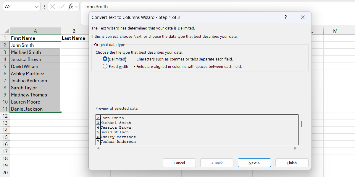
To do that, select the delimited data and click Text to Columns in the Data Tools section of the Data tab. Ensure the Delimited radio button is selected and click Next.

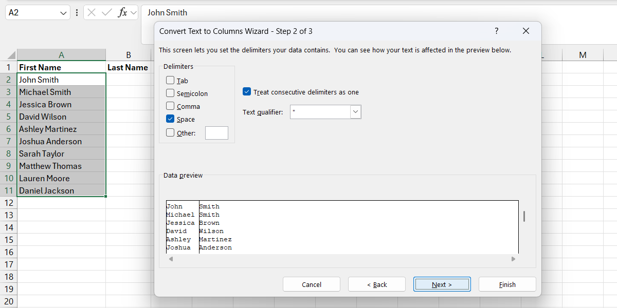
In the Delimiters section, tick the ones you want to use to split the text and click Finish.

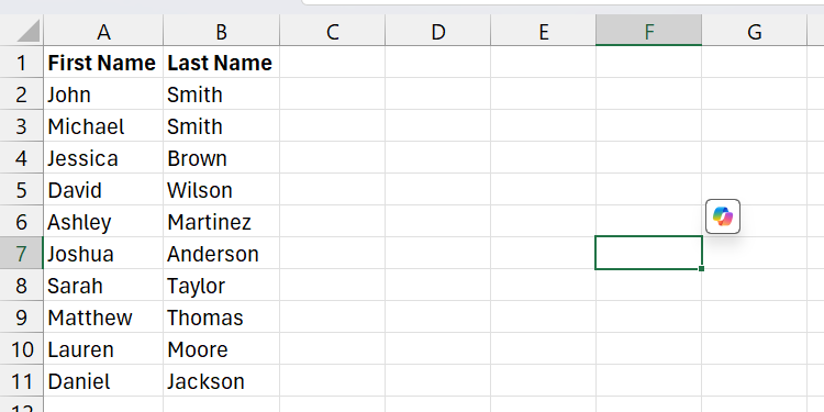
Afterward, you should see the text split into columns based on how it is delimited.

Related

How to Use the LEFT, RIGHT, and MID Functions in Excel

Extract specific strings from your Excel cells using these functions.

These Excel tips can transform a chaotic spreadsheet into a well-organized, professional document. By implementing these simple yet effective techniques, you’ll save time, reduce errors, and make your data more reliable and easier to analyze.